FunSAS
This page references the official documentation of FunSAS.
Method Description
The article introduces a novel model-based procedure for sparse clustering of functional data, referred to as Sparse and Smooth Functional Clustering. It is referred to as SaS-Funclust in the paper, but for the sake of naming consistency in our package, it is denoted as FunSAS. This method is designed to classify a set of curves into homogeneous groups while also identifying the most informative parts of the domain. Here’s a concise description of the method:
Objective function
The method aims to enhance both the accuracy and interpretability of functional data clustering by detecting informative portions of the domain.
Model
It relies on a functional Gaussian mixture model, where parameters are estimated by maximizing a log-likelihood function penalized with a functional adaptive pairwise fusion penalty and a roughness penalty.
Penalties
Functional Adaptive Pairwise Fusion Penalty (FAPFP): This penalty identifies noninformative portions of the domain by allowing the means of separated clusters to converge to common values.
Smoothness Penalty
This penalty imposes a degree of smoothing on the estimated cluster means to improve interpretability.
Algorithm
The model is estimated using an Expectation-Conditional Maximization (ECM) algorithm paired with a cross-validation procedure for parameter selection.
Performance
Through a Monte Carlo simulation study, SaS-Funclust outperforms other methods in terms of clustering performance and interpretability.
Function
This method provides five core functions: sas_sim_data for simulation module, sas_bifunc and sas_bifunc_cv for modeling module, FDPlot.sas_fdplot and FDPlot.sas_cvplot for visualization module. Because the parameters of functions sas_bifunc and sas_bifunc_cv are similar while their outputs differ, we will explain the two functions together.
sas_sim_data
sas_sim_data generates simulated data in different scenarios.
sas_sim_data(scenario, n_i = 50, nbasis = 30, length_tot = 50, var_e = 1, var_b = 1, seed = 123)
Parameter
Parameter |
Description |
|---|---|
scenario |
integer 0, 1 or 2, a number indicating the scenario considered, which stands for “Scenario I”, “Scenario II”, and “Scenario III” respectively. |
n_i |
integer, number of curves in each cluster. Default is 50. |
nbasis |
integer, the dimension of the set of B-spline functions. Default is 30. |
length_tot |
integer, number of evaluation points. Default is 50. |
var_e |
integer, variance of the measurement error. Default is 1. |
var_b |
integer, diagonal entries of the coefficient variance matrix, which is assumed to be diagonal, with equal diagonal entries, and the same among clusters. |
seed |
integer, random seeds each time when data is generated. Default is 123. |
Value
The function sas_sim_data outputs a dict contains following arguments:
X: observation matrix, where the rows correspond to argument values and columns to replications.
X_fd: functional observations without measurement error.
mu_fd: true cluster mean function.
grid: the vector of time points where the curves are sampled.
clus: true cluster membership vector.
Example
from BiFuncLib.simulation_data import sas_sim_data
sas_simdata = sas_sim_data(1, n_i = 20, var_e = 1, var_b = 0.25)
sas_bifunc & sas_bifunc_cv
cc_bifunc performs model fitting, while cc_bifunc_cv performs K-fold cross-validation procedure to choose the number of clusters and the tuning parameters for the model.
sas_bifunc(X = None, timeindex = None, curve = None, grid = None, q = 30, par_LQA = None,
           lambda_l = 1e1, lambda_s = 1e1, G = 2, tol = 1e-7, maxit = 50, plot = False,
           trace = False, init = "kmeans", varcon = "diagonal", lambda_s_ini = None)
and
sas_bifunc_cv(X = None, timeindex = None, curve = None, grid = None, q = 30,
              lambda_l_seq = None, lambda_s_seq = None, G_seq = None, tol = 1e-7, maxit = 50,
              par_LQA = None, plot = False, trace = False, init = "kmeans", varcon = "diagonal",
              lambda_s_ini = None, K_fold = 5, X_test = None, grid_test = None, m1 = 1, m2 = 0, m3 = 1)
Parameter
Parameter |
Description |
|---|---|
X |
array, observation matrix, where the rows correspond to argument values and columns to replications. |
timeindex |
array or none, a vector of length \(\sum_{i=1}^{N} n_i\). The entries from \(\sum_{i=1}^{k-1}(n_i+1)\) to \(\sum_{i=1}^{k} n_i\) provide the locations on grid of curve \(k\). Default is None. |
curve |
array or none, a vector of length \(\sum_{i=1}^{N} n_i\). The entries from \(\sum_{i=1}^{k-1}(n_i + 1)\) to \(\sum_{i=1}^{k} n_i\) are equal to \(k\). If X is a matrix, curve is ignored. Default is None. |
grid |
array or none, the vector of time points where the curves are sampled. |
q |
numeric, the dimension of the set of B-spline functions. Default is 30. |
par_LQA |
dict or none, parameters for the local quadratic approximation (LQA) in the ECM algorithm. eps_diff is the lower bound for the coefficient mean differences, values below eps_diff are set to zero. MAX_iter_LQA is the maximum number of iterations allowed in the LQA. eps_LQA is the tolerance for the stopping condition of LQA. If none, default is par_LQA = {“eps_diff”: 1e-6, “MAX_iter_LQA”: 200, “eps_LQA”: 1e-5}. |
lambda_l/lambda_l_seq |
numeric/array, number/sequence of tuning parameter of the functional adaptive pairwise fusion penalty (FAPFP). |
lambda_s/lambda_s_seq |
numeric/array, number/sequence of tuning parameter of the smoothness penalty. |
G/G_seq |
integer/array, number/sequence of number of clusters |
tol |
numeric, the tolerance for the stopping condition of the expectation conditional maximization (ECM) algorithms. Default is 1e-7. |
maxit |
integer, the maximum number of iterations allowed in the ECM algorithm. Default is 50. |
plot |
bool, if True, the estimated cluster means are plotted at each iteration of the ECM algorithm. Default is False. |
trace |
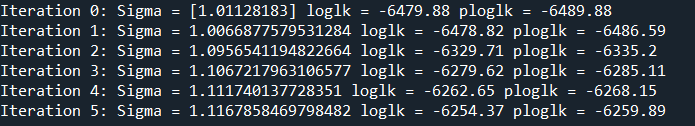
bool, if True, information are shown at each iteration of the ECM algorithm. Default is False. |
init |
str, the way to initialize the ECM algorithm. There are three ways of initialization: ‘kmeans’, ‘model-based’, and ‘hierarchical’, that provide initialization through the k-means algorithm, model-based clustering based on parameterized finite Gaussian mixture model, and hierarchical clustering, respectively. Default is “kmeans”. |
varcon |
str, the type of coefficient covariance matrix. Three values are allowed: “full”, “diagonal”, and “equal”. “full” means unrestricted cluster coefficient covariance matrices allowed to be different among clusters. “diagonal” means diagonal cluster coefficient covariance matrices that are equal among clusters. “equal” means diagonal cluster coefficient covariance matrices, with equal diagonal entries, that are equal among clusters. Default is “diagonal”. |
lambda_s_ini |
numeric or none, The tuning parameter used to obtain the functional data through smoothing B-splines before applying the initialization algorithm. If none a Generalized cross validation procedure is used as described in Ramsay (2005). Default is None. |
K_fold |
integer, number of folds. Default is 5. |
X_test |
array or none, only for functional data observed over a regular grid, a matrix where the rows must correspond to argument values and columns to replications of the test set. Default is None. |
grid_test |
array or none, the vector of time points where the test set curves are sampled. Default is None. |
m1 |
numeric, the m-standard deviation rule parameter to choose G for each lambda_s and lambda_l. Default is 1. |
m2 |
numeric, the m-standard deviation rule parameter to choose lambda_s fixed G for each lambda_l. Default is 0. |
m3 |
numeric, the m-standard deviation rule parameter to choose lambda_l fixed G and lambda_s. Default is 1. |
If trace=True, it will print how each metric evolves across iterations.
Value
The function sas_bifunc outputs a dict including clustering results and information of the model.
mod 1. data: dict, contains the vectorized form of X, timeindex, and curve. For functional data observed over a regular grid timeindex and curve are trivially obtained. 2. parameters: dict, contains all the estimated parameters. 3. vars: dict contains results from the Expectation step of the ECM algorithm. 4. FullS: array, the matrix of B-spline computed over grid. 5. grid: list, the vector of time points where the curves are sampled. 6. W: array, the basis roughness penalty matrix containing the inner products of pairs of basis function second derivatives. 7. AW_vec: array, vectorized version of the diagonal matrix used in the approximation of FAPFP. 8. P_tot: sparse.csr.csr_matrix, Sparse Matrix used to compute all the pairwise comparisons in the FAPFP. 9. lambda_s: numeric, tuning parameter of the smoothness penalty. 10. lambda_l: numeric, tuning parameter of the FAPFP.
clus 1. classes: array, the cluster membership. 2. po_pr: array, posterior probabilities of cluster membership.
mean_fd: dict, the estimated cluster mean functions generated by GENetLib.
The function cc_bifunc_cv outputs clustering results and optimal parameters.
G_opt: integer, the optimal number of clusters.
lambda_l_opt: array, the optimal tuning parameter of the FAPFP.
lambda_s_opt: array, the optimal tuning parameter of the smoothness penalty.
comb_list: array, the combinations of G, lambda_s and lambda_l explored.
CV: array, the cross-validation values obtained for each combination of G,lambda_s and lambda_l.
CV_sd: array, the standard deviations of the cross-validation values.
zeros: array, fraction of domain over which the estimated cluster means are fused.
ms: tuple, the m-standard deviation rule parameters.
Example
import numpy as np
from BiFuncLib.simulation_data import sas_sim_data
from BiFuncLib.sas_bifunc import sas_bifunc, sas_bifunc_cv
sas_simdata = sas_sim_data(1, n_i = 20, var_e = 1, var_b = 0.25)
sas_result = sas_bifunc(X = sas_simdata['X'], grid = sas_simdata['grid'],
                        lambda_s = 1e-6, lambda_l = 10, G = 2, maxit = 5, q = 10,
                        init = 'hierarchical', trace = True, varcon = 'full')
lambda_s_seq = 10 ** np.arange(-4, -2, dtype=float)
lambda_l_seq = 10 ** np.arange(-1, 1, dtype=float)
G_seq = [2, 3]
sas_cv_result = sas_bifunc_cv(X = sas_simdata['X'], grid = sas_simdata['grid'],
                              lambda_l_seq = lambda_l_seq, lambda_s_seq = lambda_s_seq,
                              G_seq = G_seq, maxit = 20, K_fold = 2, q = 10)
FDPlot.sas_fdplot & FDPlot.sas_cvplot
When applied to sas_bifunc output, the FDPlot.sas_fdplot function plots the estimated cluster mean functions and the classified curves.
FDPlot(result).sas_fdplot()
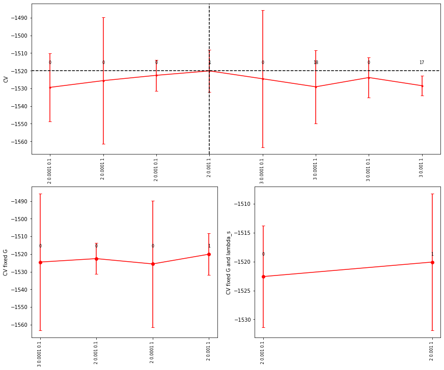
When applied to sas_bifunc_cv output, it produces cross-validation plots: the first shows CV values versus G, lambda_s, and lambda_l; the second fixes G at its optimum and shows CV values versus lambda_s and lambda_l; the third fixes both G and lambda_s at their optima and shows CV values versus lambda_l.
FDPlot(result).sas_cvplot()
Parameter
Parameter |
Description |
|---|---|
result |
dict, a clustering result generated by sas_bifunc or sas_bifunc_cv function. |
Value
FDPlot.sas_fdplot

FDPlot.sas_cvplot
Example
import numpy as np
from BiFuncLib.FDPlot import FDPlot
from BiFuncLib.simulation_data import sas_sim_data
from BiFuncLib.sas_bifunc import sas_bifunc, sas_bifunc_cv
sas_simdata_0 = sas_sim_data(1, n_i = 20, var_e = 1, var_b = 0.25)
sas_result = sas_bifunc(X = sas_simdata_0['X'], grid = sas_simdata_0['grid'],
                        lambda_s = 1e-6, lambda_l = 10, G = 2, maxit = 5, q = 10,
                        init = 'hierarchical', trace = True, varcon = 'full')
lambda_s_seq = 10 ** np.arange(-4, -2, dtype=float)
lambda_l_seq = 10 ** np.arange(-1, 1, dtype=float)
G_seq = [2, 3]
sas_cv_result = sas_bifunc_cv(X = sas_simdata_0['X'], grid = sas_simdata_0['grid'],
                              lambda_l_seq = lambda_l_seq, lambda_s_seq = lambda_s_seq,
                              G_seq = G_seq, maxit = 20, K_fold = 2, q = 10)
FDPlot(sas_result).sas_fdplot()
FDPlot(sas_cv_result).sas_cvplot()