FunLocal
Method Description
This method is developed by our team. We proposed a method named Local Clustering for Functional Data (LFC), which is a penalized-model-based local-clustering method that extends traditional functional clustering by allowing different clustering structures in different continuous sub-intervals of the domain. It is particularly suited to longitudinal/functional data whose underlying heterogeneity varies over the measurement domain (e.g., COVID-19 case trajectories across U.S. states). Key methodological stages are listed below.
Functional representation
Each observed curve is projected onto a B-spline basis expansion, yielding a finite-dimensional coefficient vector. The compact support of B-splines is later exploited to perform local fusion without reconstructing the whole curve.
Model definition (Local Functional Clustering)
Global clusters: a single partition of all n individuals over the entire domain T.
Local clusters: M non-overlapping sub-intervals with potentially different partitions of the n individuals in each sub-interval.
Parameters: block-specific B-spline coefficient vectors (means) and their associated covariance structures.
Penalty: a three-part regularization, (i) spline roughness penalty for smoothness; (ii) individual-to-centre fusion for global clustering; (iii) local centre-to-centre fusion that automatically discovers the sub-intervals T_m and the corresponding local cluster partitions.
Model inference (ADMM-proximal algorithm)
An Alternating Direction Method of Multipliers (ADMM) framework is adopted, embedding a nested FISTA/proximal-average step to handle the non-convex MCP fusion penalties efficiently.
Model selection
The smoothing parameter is chosen by Generalized Cross Validation (GCV). Clustering and sparsity parameters are selected via a modified Bayesian Information Criterion (mBIC), which also determines the number of global clusters, the number of local clusters in each sub-interval, and the number of sub-intervals M.
Visualization and interpretation
Estimated global and local cluster mean curves are plotted together with raw curves for each identified group. A temporal segmentation plot highlights the discovered sub-intervals and their associated cluster patterns, enabling domain-driven interpretation.
Function
This method provides four core functions: local_sim_data, local_bifunc, FDPlot.local_individuals_fdplot and FDPlot.local_center_fdplot for visualization. In this section, we detail their respective usage, as well as parameters, output values and usage examples for each function.
local_sim_data
local_sim_data generates simulated data according to the FunLocal model.
local_sim_data(n, T, sigma, seed = 123)
Parameter
Parameter |
Description |
|---|---|
n |
integer, the number of samples. |
T |
integer, the number of time points per sample. |
sigma |
numeric, the noise level added to the data. A higher value of sigma introduces more random variation, making the clustering task more challenging. |
seed |
integer, random seeds each time when data is generated. Default is 123. |
Value
The function local_sim_data outputs a dict contains simulated data matrix and the true clustering results.
data: dataframe, a simulated data with different time and measurements.
location: array, a sequence of time from 0 to 1.
sample cluster: list, true sample clustering results.
Example
from BiFuncLib.simulation_data import local_sim_data
local_simdata = local_sim_data(n = 100, T = 100, sigma = 0.75, seed = 1)
local_bifunc
local_bifunc performs model fitting, including optimization for tuning parameters.
local_bifunc(data, times, lambda1, lambda2, lambda3, opt = False, rangeval = (0, 1), nknots = 30, order = 4,
             nu = 2, tau = 3, K0 = 6, rep_num = 100, kappa = 1, eps_outer = 0.0001, max_iter = 100)
Parameter
In this part, if the parameters lambda1, lambda4, and lambda3 are individual values, then opt should be set to False, which means the model is established with fixed parameters. If all three parameters are sequences (even if one parameter does not need to find the optimal value, it should still be written in the form of a sequence), then opt should be set to True, which allows the model to automatically search for the optimal parameters.
Parameter |
Description |
|---|---|
data |
dataframe, the input functional data matrix. Each row typically represents an individual curve, and each column represents a measurement at a specific time point. |
times |
array, the time points at which the data is observed. This is a vector of length equal to the number of columns in data. |
lambda1 |
numeric or array, the smoothing parameter for the B-spline basis expansion. Controls the smoothness of the estimated curves. |
lambda2 |
numeric or array, the clustering penalty parameter. Controls the strength of the clustering regularization. |
lambda3 |
numeric or array, the sparsity penalty parameter. Controls the strength of the sparsity regularization. |
opt |
bool, whether to perform optimization for tuning parameters. If True, the function may automatically select optimal values for lambda1, lambda2, and lambda3. |
rangeval |
tuple or numeric, a tuple specifying the range of the time domain. Default is (0, 1). |
nknots |
integer, the number of interior knots for the B-spline basis. Determines the flexibility of the spline approximation. Default is 30. |
order |
integer, the order of the B-spline basis. Higher orders provide smoother curves. Default is 4. |
nu |
integer, the order of the differential operator used in the smoothing penalty. Default is 2. |
tau |
integer, the threshold parameter for the MCP (Minimax Concave Penalty) used in the clustering and sparsity penalties. Default is 3. |
K0 |
integer, an initial upper bound for the number of global clusters. This helps in determining the maximum number of clusters to consider. Default is 6. |
rep_num |
integer, the number of replications for the algorithm. This can be used to ensure stability and robustness of the clustering results. Default is 100. |
kappa |
numeric, a small positive constant used in the ADMM algorithm for convergence control. Default is 1. |
eps_outer |
numeric, the convergence tolerance for the outer loop of the ADMM algorithm. Smaller values ensure more precise convergence. Default is 0.0001. |
max_iter |
integer, the maximum number of iterations for the ADMM algorithm. Default is 100. |
Value
The function local_bifunc outputs a dict including clustering results and information of the model.
basisobj: dict, stands for the B-spline basis.
Beta: array, the estimated B-spline coefficients.
Beta_ini: array, the initial estimates of the B-spline coefficients.
centers: integer, the B-spline coefficients for two cluster centers.
cls_mem: array, the cluster membership (0 or 1) for each of the data points.
cls_num: int, the number of clusters identified.
lambda1_opt: numeric, the optimized smoothing parameter.
lambda2_opt: numeric, the optimized clustering parameter.
lambda3_opt: numeric, the optimized sparsity parameter.
Example
import numpy as np
from BiFuncLib.local_bifunc import local_bifunc
from BiFuncLib.simulation_data import local_sim_data
local_simdata = local_sim_data(n = 100, T = 100, sigma = 0.75, seed = 1)
res = local_bifunc(local_simdata['data'], local_simdata['location'],
                  1.02e-5, 2, 0.3, opt=False)
opt_res = local_bifunc(local_simdata['data'], local_simdata['location'],
                      np.array([1.02e-5]), np.array([2,3]), np.array([0.3,0.5]), opt=True)
FDPlot.local_individuals_fdplot & FDPlot.local_center_fdplot
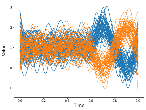
FDPlot.local_individuals_fdplot displays the raw functional data for all individuals, color-coded by their cluster membership as identified by the method.
FDPlot(opt_res).local_individuals_fdplot()
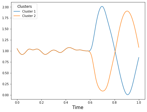
FDPlot.local_center_fdplot visualizes the estimated mean curves for two distinct clusters identified by the method.
FDPlot(opt_res).local_center_fdplot()
Parameter
Parameter |
Description |
|---|---|
result |
dict, a clustering result generated by pf_bifunc function. |
Value
Raw functional data
Estimated mean curves
Example
from BiFuncLib.FDPlot import FDPlot
import numpy as np
from BiFuncLib.local_bifunc import local_bifunc
from BiFuncLib.simulation_data import local_sim_data
local_simdata = local_sim_data(n = 100, T = 100, sigma = 0.75, seed = 1)
res = local_bifunc(local_simdata['data'], local_simdata['location'],
                  1.02e-5, 2, 0.3, opt=False)
opt_res = local_bifunc(local_simdata['data'], local_simdata['location'],
                      np.array([1.02e-5]), np.array([2,3]), np.array([0.3,0.5]),
                      opt=True)
FDPlot(opt_res).local_individuals_fdplot()
FDPlot(opt_res).local_center_fdplot()