FunLBM
This page references the official documentation of FunLBM.
Method Description
FunLBM is a model-based co-clustering method specifically designed for functional data, such as high-frequency electricity consumption curves. It extends the traditional Latent Block Model (LBM) to handle functional data by assuming that the curves within each block live in a low-dimensional functional subspace. This approach enables the co-clustering of both individuals (e.g., households) and features (e.g., days of observation) to provide meaningful summaries of large datasets. The key steps of the method are:
Functional Data Representation
Each observed curve is first smoothed using a basis expansion (e.g., Fourier basis), converting discrete observations into continuous functional forms. This step ensures that the data are represented in a functional subspace suitable for co-clustering.
Model Definition (Functional LBM)
The Functional LBM assumes that the curves within each block can be adequately described in a low-dimensional latent subspace. The model parameters include block-specific means, variances, and covariance matrices, which are estimated to capture the underlying structure of the data.
Model Inference (SEM-Gibbs Algorithm)
An iterative Stochastic Expectation-Maximization (SEM) algorithm embedded with Gibbs sampling is used for model inference. The algorithm alternates between:
SE Step: Generate the unobserved row and column partitions using Gibbs sampling.
Maximization Step: Update the model parameters based on the generated partitions.
Model Selection
The optimal number of row and column groups (K and L) is selected using the Integrated Completed Likelihood (ICL) criterion. This criterion balances model complexity and fit to the data, ensuring that the chosen model provides the best trade-off between parsimony and accuracy.
Visualization and Interpretation
The co-clustering results are visualized through estimated functional means and proportions of row and column groups. This allows for an interpretable summary of the data, highlighting patterns and behaviors within different clusters.
Function
This method provides three core functions: lbm_sim_data, lbm_bifunc and FDPlot.lbm_fdplot. In this section, we detail their respective usage, as well as parameters, output values and usage examples for each function.
lbm_sim_data
lbm_sim_data generates simulated data according to the funLBM model with K=4 groups for rows and L=3 groups for columns.
lbm_sim_data(n = 100, p = 100, t = 30, bivariate = False, noise = None, seed = 111)
Parameter
Parameter |
Description |
|---|---|
n |
integer, the number of rows (individuals) of the simulated data array. |
p |
integer, the number of columns (functional variables) of the simulated data array, |
t |
integer, the number of measures for the functions of the simulated data array. |
bivariate |
bool, whether to generate bivariate simulated data. Default is False. |
noise |
numeric or None, the noise intensity of simulated data. Default is 0. |
seed |
integer, random seeds each time when data is generated. Default is 111. |
Value
The function lbm_sim_data has two types of outputs: one is non-bivariate data, which is a three-dimensional matrix; the other is bivariate data, which includes two three-dimensional matrices.
data: array, if bivariate=False, outputs data array of size n x p x t. If bivariate=True, outputs two distinct n x p x t datasets.
row_clust: array, group memberships of rows for evaluation.
col_clust: array, group memberships of columns for evaluation.
Example
from BiFuncLib.simulation_data import lbm_sim_data
lbm_simdata1 = lbm_sim_data(n = 100, p = 100, t = 30, seed = 1)
data1 = lbm_simdata1['data']
lbm_simdata2 = lbm_sim_data(n = 50, p = 50, t = 15, bivariate = True)
data2 = [lbm_simdata2['data1'],lbm_simdata2['data2']]
lbm_bifunc
lbm_bifunc performs model fitting.
lbm_bifunc(data, K, L, maxit = 50, burn = 25, basis_name = 'fourier', nbasis = 15, gibbs_it = 3, display = False, init = 'funFEM')
Parameter
Parameter |
Description |
|---|---|
data |
array or list, a data array of size n x p x t or a list contains two distinct n x p x t datasets. |
K |
integer or list, the number of row clusters. If It is a list, the function performs grid search for best K. |
L |
integer or list, the number of column clusters. If It is a list, the function performs grid search for best L. |
maxit |
integer, the maximum number of iterations of the SEM-Gibbs algorithm. Default is 50. |
burn |
integer, the number of of iterations of the burn-in period. Default is 25. |
basis_name |
str, the name(‘fourier’ or ‘spline’) of the basis functions used for the decomposition of the functions. Default is ‘fourier’. |
nbasis |
integer, number of the basis functions used for the decomposition of the functions. Default is 15. |
gibbs_it |
integer, number of Gibbs iterations. Default is 3. |
display |
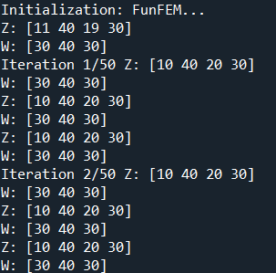
bool, if true, information about the iterations is displayed. Default is False. |
init |
str, the type of initialization: ‘random’, ‘kmeans’ or ‘funFEM’. Default is ‘funFEM’. |
Value
The function lbm_bifunc outputs a dict including clustering results and information of the model.
prms: dict, a dict containing all fitted parameters for the best model (according to ICL).
Z: array, the dummy matrix of row clustering.
W: array, the dummy matrix of column clustering.
row_clust: list, the group memberships of rows.
col_clust: liat, the group memberships of columns.
allPrms: dict, a dict containing the fitted parameters for all tested models.
loglik: array, an array contains all the log-likelihood of the iterations.
icl: numeric, the value of ICL for the best model.
allRes: list, if perform grid search for K and L, the function outputs information for all the models.
criteria: list, if perform grid search for K and L, the function outputs the ICL value for each model.
If display=True, the following information will be returned.
Example
from BiFuncLib.simulation_data import lbm_sim_data
from BiFuncLib.lbm_bifunc import lbm_bifunc
from BiFuncLib.lbm_main_func import ari
lbm_simdata1 = lbm_sim_data(n = 100, p = 100, t = 30, seed = 1)
data1 = lbm_simdata1['data']
lbm_res = lbm_bifunc(data1, K=4, L=3, display=True, init = 'kmeans')
print(ari(lbm_res['col_clust'],lbm_simdata1['col_clust']))
print(ari(lbm_res['row_clust'],lbm_simdata1['row_clust']))
# Grid search for K
lbm_simdata2 = lbm_sim_data(n = 50, p = 50, t = 15, bivariate = True)
data2 = [lbm_simdata2['data1'],lbm_simdata2['data2']]
lbm_res_grid = lbm_bifunc(data2, K=[2,3,4], L=[2,3], init = 'funFEM')
print(ari(lbm_res_grid['col_clust'],lbm_simdata2['col_clust']))
print(ari(lbm_res_grid['row_clust'],lbm_simdata2['row_clust']))
It is worth noting that the ari function computes the Adjusted Rand Index (ARI), which compares two clustering partitions to evaluate the accuracy of the model’s classification. The function takes two sequences (lists or arrays) as input and returns a value between 0 and 1; the closer this value is to 1, the better the agreement between the two partitions.
FDPlot.lbm_fdplot
FDPlot.lbm_fdplot produces various kinds of visualizations.
FDPlot(result).lbm_fdplot(data, types='blocks')
Parameter
Parameter |
Description |
|---|---|
result |
dict, a clustering result generated by lbm_bifunc function. |
types |
str, The type of plot to display. Possible plots are ‘blocks’ (default), ‘means’, ‘evolution’, ‘likelihood’ and ‘proportions’. |
Value
Here we illustrate the outputs of the plot function under different class configurations.
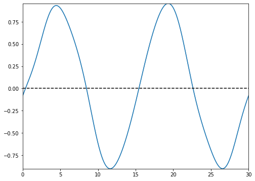
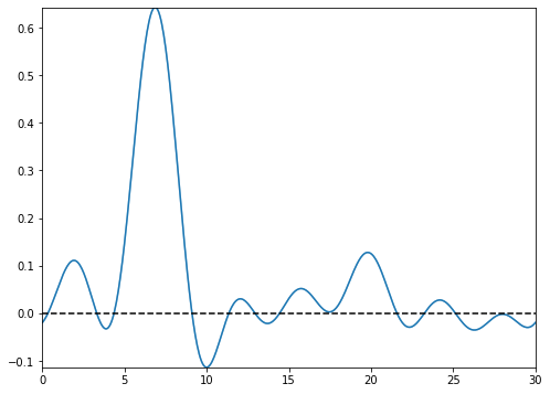
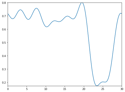
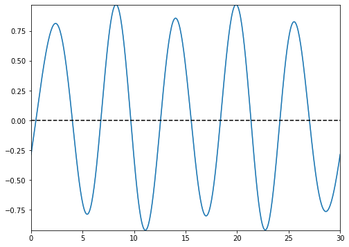
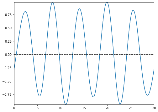
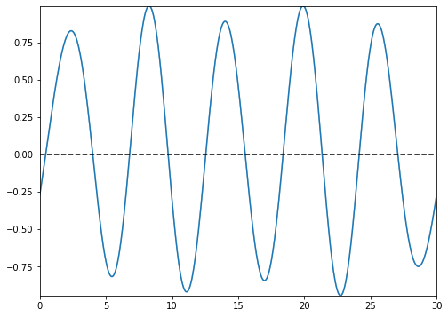
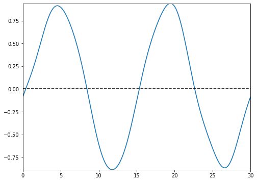
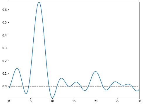
types=’blocks’
This setting outputs the functional images of the block matrix.
|
|
|
|
|
|
|
|
|
|
|
|


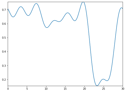
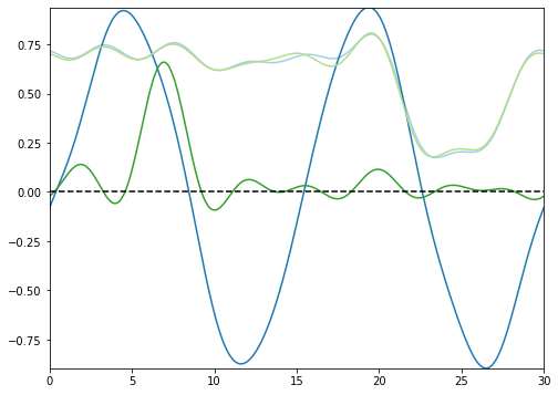
types=’means’
This setting outputs the functional images of the estimated functional means.
|
|
|


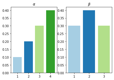
types=’proportions’
This setting outputs the row and column mixing proportions respectively.
types=’evolution’
This setting outputs the evolution of the SEM-Gibbs estimates for model parameters along the iterations.

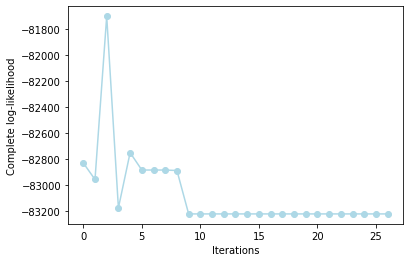
types=’likelihood’
This setting outputs the behaviour of the complete-data likelihood over the iterations of the functional LBM algorithm.
Example
from BiFuncLib.FDPlot import FDPlot
from BiFuncLib.simulation_data import lbm_sim_data
from BiFuncLib.lbm_bifunc import lbm_bifunc
lbm_simdata1 = lbm_sim_data(n = 100, p = 100, t = 30, seed = 12)
data1 = lbm_simdata1['data']
lbm_res = lbm_bifunc(data1, K=4, L=3, display=False, init='kmeans')
FDPlot(lbm_res).lbm_fdplot('proportions')
FDPlot(lbm_res).lbm_fdplot('evolution')
FDPlot(lbm_res).lbm_fdplot('likelihood')
FDPlot(lbm_res).lbm_fdplot('blocks')
FDPlot(lbm_res).lbm_fdplot('means')