FunPF
Method Description
This method is developed by our team. We propose a doubly-penalized fusion framework that simultaneously estimates smooth functional curves and discovers row (sample) and column (covariate) clusters in a single optimization. The method is distribution-free and automatically determines the number of clusters. The key steps are listed below.
Functional Representation
Each observed curve is expanded with B-spline basis functions
\[g_{i,j}(t) \approx \mathbf{U}_p(t)^\top \boldsymbol{\beta}_{i,j},\]yielding coefficient vectors \(\boldsymbol{\beta}_{i,j} \in \mathbb{R}^p\).
Objective Function
Minimize
\[L(\boldsymbol{\beta}) = \frac{1}{2}\| \mathbf{Y} - \mathbf{U} \boldsymbol{\beta} \|_2^2 + \frac{\gamma_1}{2} \boldsymbol{\beta}^\top \mathbf{M} \boldsymbol{\beta} + \gamma_2 \sum_{i_1 < i_2} \rho_\tau \left( \| \boldsymbol{\beta}^{(r)}_{i_1} - \boldsymbol{\beta}^{(r)}_{i_2} \|_2 \right) + \gamma_2 \sqrt{\frac{N}{q}} \sum_{j_1 < j_2} \rho_\tau \left( \| \boldsymbol{\beta}^{(c)}_{j_1} - \boldsymbol{\beta}^{(c)}_{j_2} \|_2 \right),\]
where
\(\gamma_1\) smooths each curve via a second-order difference penalty (matrix \(\mathbf{M}\));
\(\gamma_2\) induces fusion of sample / covariate coefficients via a concave penalty \(\rho_\tau\) (MCP or SCAD);
\(\boldsymbol{\beta}^{(r)}_i\) and \(\boldsymbol{\beta}^{(c)}_j\) denote the stacked coefficients for sample \(i\) and covariate \(j\) respectively.
Tuning
Step 1 (smoothness): fix \(\gamma_2 = 0\) and choose optimal \(\gamma_1\) via BIC.
Step 2 (fusion): fix \(\gamma_1\) and choose \(\gamma_2\) via a second BIC.
ADMM Algorithm
Primal updates: closed-form ridge-type solution for \(\boldsymbol{\beta}\).
Dual updates: closed-form soft-thresholding for sample- and covariate-level fusion variables.
Convergence: monitored through primal and dual residuals.
Statistical Guarantees
Consistency: under mild regularity, the oracle estimator (with known clusters) achieves
\[\| \hat{g}_{k_r,k_c} - g^*_{k_r,k_c} \| = O_P \left( \left( \frac{p \log(Nq)}{|G_{\min}|} \right)^{1/2} \right).\]Clustering consistency: a local minimizer equals the oracle estimator with probability → 1 as \(N, q \to \infty\).
Function
This method provides three core functions: pf_sim_data, pf_bifunc and FDPlot.pf_fdplot. In this section, we detail their respective usage, as well as parameters, output values and usage examples for each function.
pf_sim_data
pf_sim_data generates simulated data according to the FunPF model, which transforms the 3D data into a 2D matrix, and seperates data into 3*3 parts.
pf_sim_data(n, T, nknots, order, seed = 123)
Parameter
Parameter |
Description |
|---|---|
n |
integer, the number of samples. |
T |
integer, the number of time points per sample. |
nknots |
integer, the number of interior knots used in the B-spline basis expansion for estimating the underlying mean functions. |
order |
integer, the polynomial degree of the B-spline basis plus one (e.g., order 4 gives cubic splines). |
seed |
integer, random seeds each time when data is generated. Default is 123. |
Value
The function pf_sim_data outputs a dict contains simulated data matrix and the true clustering results.
data: dataframe, a simulated data with different time and measurements.
location: array, a sequence of time from 0 to 1.
feature cluster: list, true feature clustering results.
sample cluster: list, true sample clustering results.
Example
from BiFuncLib.simulation_data import pf_sim_data
pf_simdata = pf_sim_data(n = 60, T = 10, nknots = 3, order = 3, seed = 123)['data']
pf_bifunc
pf_bifunc performs model fitting.
pf_bifunc(data, nknots, order, gamma1, gamma2, opt = False, theta = 1, tau = 3, max_iter = 500, eps_abs = 1e-3, eps_rel = 1e-3)
Parameter
Parameter |
Description |
|---|---|
data |
array or list, a data array of size n x p x t or a list contains two distinct n x p x t datasets. |
nknots |
integer, number of interior knots used in the B-spline basis expansion for estimating the underlying mean functions. |
order |
integer, polynomial degree of the B-spline basis plus one (e.g., order 4 gives cubic splines). |
gamma1 |
numeric or list, smoothness penalty tuning parameter that controls the trade-off between data fidelity and functional smoothness during estimation. |
gamma2 |
numeric or list, fusion penalty tuning parameter that governs the strength of clustering by penalizing differences between coefficient vectors. |
opt |
bool, if True the function selects optimal (gamma1, gamma2) via a two-step BIC procedure; otherwise user-supplied values are used. Default is False. |
theta |
numeric (>0), ADMM augmented-Lagrangian penalty weight. Default is 1. |
tau |
numeric (>1), MCP/SCAD regularization parameter controlling the concavity of the fusion penalty. Default is 3. |
max_iter |
integer, maximum number of ADMM iterations before stopping. Default is 500. |
eps_abs |
numeric (>0), absolute convergence tolerance for primal and dual residuals. Default is 1e-3. |
eps_rel |
numeric (>0), relative convergence tolerance for primal and dual residuals. Default is 1e-3. |
Value
The function pf_bifunc outputs a dict including clustering results and information of the model. The key results are feature_cluster and sample_cluster, and we omitted the outputs that are identical to the inputs.
Beta: list, estimated regression coefficients for each covariate in the model.
feature_cluster: list, the clustering assignment for each feature or covariate.
feature_number: integer, the total count of features or covariates considered in the analysis.
iter: integer, the number of iterations the algorithm has executed.
Lambda1: numeric, the Lagrange multipliers associated with the row clustering constraints.
Lambda2: numeric, the Lagrange multipliers related to the column clustering constraints.
sample_cluster: list, the clustering assignment for each sample or observation.
sample_number: integer, the total number of samples or observations in the dataset.
Example
from BiFuncLib.simulation_data import pf_sim_data
pf_simdata = pf_sim_data(n = 60, T = 10, nknots = 3, order = 3, seed = 123)['data']
pf_result = pf_bifunc(pf_simdata, nknots = 3, order = 3, gamma1 = 0.023, gamma2 = 3,
                      theta = 1, tau = 3, max_iter = 500, eps_abs = 1e-3, eps_rel = 1e-3)
# Performs opt
pf_result_opt = pf_bifunc(pf_simdata, nknots = 3, order = 3, gamma1 = [0.023, 0.025], gamma2 = [2,3],
                          opt = True, theta = 1, tau = 3, max_iter = 500, eps_abs = 1e-3, eps_rel = 1e-3)
FDPlot.pf_fdplot
FDPlot.pf_fdplot visualizes the result generated by pf_bifunc function.
FDPlot(result).pf_fdplot()
Parameter
Parameter |
Description |
|---|---|
result |
dict, a clustering result generated by pf_bifunc function. |
Value
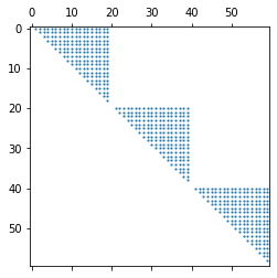
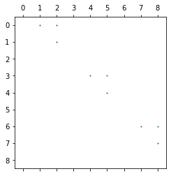
The function has two parts of output. One is the lattice plot of the clustering results, and the other is the reconstructed function curves.
Lattice plot of the clustering results
|
|
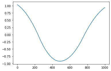
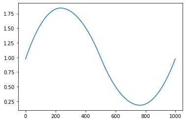
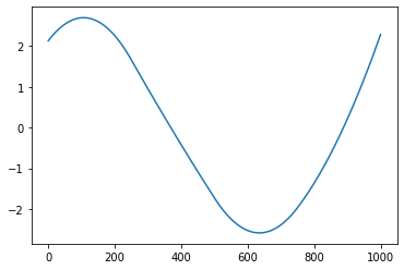
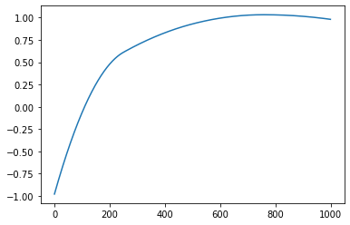
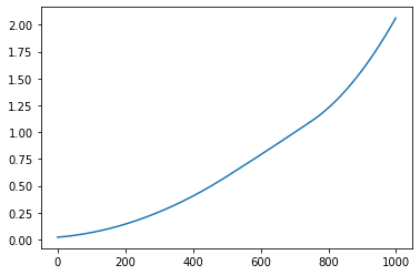
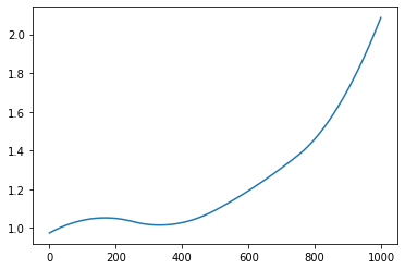
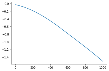
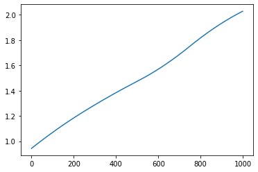
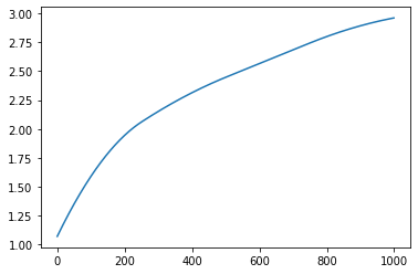
Reconstructed function curves
|
|
|
|
|
|
|
|
|
Example
from BiFuncLib.pf_bifunc import pf_bifunc
from BiFuncLib.simulation_data import pf_sim_data
from BiFuncLib.FDPlot import FDPlot
pf_simdata = pf_sim_data(n = 60, T = 10, nknots = 3, order = 3, seed = 123)['data']
pf_result = pf_bifunc(pf_simdata, nknots = 3, order = 3, gamma1 = 0.023, gamma2 = 3,
                     theta = 1, tau = 3, max_iter = 500, eps_abs = 1e-3, eps_rel = 1e-3)
FDPlot(pf_result).pf_fdplot()